Epsilon and Delta in Error Models

The most common error model is that an operation x * y (taking * to be addition, subtraction, multiplication, or division, and sometimes square root or fused multiply-add) can be modeled with:

\[ x \hat{*} y = (x * y) (1 + \varepsilon) \]

Here, \(\hat{*}\) represents floating-point *, and \(\varepsilon\) represents the specific rounding error at the inputs \(x, y\), and is taken to be existentially quantified and bounded by (say) machine epsilon, about 10^-16, which I will write \(\epsilon\). Uhh, yes, it's confusing to use two different epsilons to mean two different things. There are three things here: the \(\varepsilon\) for a particular input; the bound on \(\varepsilon\) values, which depends on the operation in question; and the machine epsilon \(\epsilon\), which might be the bound on \(\varepsilon\) for some operations. Typically we elide the difference between them—I know, I know, super confusing—and I'll do that here. But the distinction is important to keep in mind; see my early post on FPTaylor for a longer description.

One way to think about \(\varepsilon\) is as the maximum relative error of your computation.

This error model is not perfect: it does not describe error cases, overflow, or underflow. These need to be checked and handled separately by automated tools—for example, an automated tool might want to check for division by zero or square root of a negative number.

Alternatively, some authors use a slightly more complicated error model with two parameters:

\[ x \hat{*} y = (x * y) (1 + \varepsilon) + \delta \]

Here \(\varepsilon\) is still bounded by machine epsilon, while \(\delta\) is bounded by the minimum positive float, about 5e-324. In this error model, \(\delta\) handles underflow. In other words, if the correct answer is \(5e-324\) but your operator returns \(0\), instead of thinking of that as a large relative error, you think of it as a tiny absolute error. Note that \(\delta\) is miniscule compared to \(\varepsilon\), and even compared to \(\varepsilon^2\). This justifies usual practice of ignoring it.

One important role of \(\delta\) and \(\varepsilon\) is that they characterize the error of a floating-point operator. Two number systems, for example, can be compared by comparing their \(\varepsilon\) and \(\delta\) parameters.

For the basic arithmetic operators, the difference between these two error models is typically small. Underflow is impossible for addition and subtraction (due to Sterbenz's lemma) and for multiplication and division it requires truly massive operands like 1e160 which are usually not of interest.

But fundamentally, this is because the basic arithmetic operators only produce zero outputs for zero inputs. Other functions are not so lucky.

Consider log, which has a zero at 1. How can we characterize its error? Well, consider the input \(x = 1 + \frac12\epsilon\), which rounds down to 1. Its exact logarithm is pretty close to \(\frac12\epsilon\), a totally reasonable floating-point value very far from underflowing or anything similar. But since \(x\) rounds down to 1, the computed logarithm is 0, giving us a 100% relative error in the first, \(\varepsilon\) error model. On the other hand, in the second, \((\varepsilon, \delta)\) error model we can characterize the error of a correctly-rounded logarithm with \(\varepsilon = \frac12\epsilon\) and \(\delta = \frac12\).

Alternatively, consider sin, which has a zero at \(\pi\). But \(\pi\) is not an exact floating-point number, and sin of that value is not exactly 0. So instead of the true value of 0, we have some non-zero value—an infinite relative error! Again, the \(\delta\) parameter adds the flexibility necessary to deal with this.

One surprising consequence of this: for arithmetic operators, \(\varepsilon\) is typically on the order of 1e-16, while \(\delta\) is on the order of 1e-324. But for functions with zeros somewhere other than at zero, \(\delta\) and \(\varepsilon\) are typically of similar order. So ignoring \(\delta\) for arithmetic functions is the unusual special case, and in general both \(\varepsilon\) and \(\delta\) are necessary, and it makes sense to discard higher-order terms while keeping first-order terms in both \(\varepsilon\) and \(\delta\).

While the intention is that \(\delta\) is only nonzero for subnormal outputs, that's not how the model is written: it allows each point to have absolute or¹ [¹ In some formalizations, the condition \(\varepsilon \delta = 0\) is added, which basically makes the relative and absolute error mutually exclusive. In practice, it's often hard to make use of this constraint in automated tools because it is highly non-convex, and fundamentally it can only make your error twice as high, which is not a big change. My point here applies regardless] relative error, at its (non-deterministic) choice.

That means typically a single operator can be characterized by multiple \((\varepsilon, \delta)\) pairs. Imagine all possible inputs to an operator, and their relative and absolute error. Some inputs have huge relative error—like 1e-300 * 1e-300, which has a relative error of 100%—while others have low relative error. Some inputs have huge absolute error—like 1e150 * 1e150—while others have low absolute error.

Now imagine the following diagram: for each input, plot a point whose horizontal and vertical positions are given by its absolute and relative error. It will look something like this:

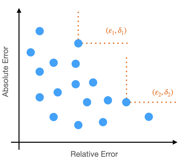
Now, some points have low absolute and relative error (some might have no error, for example!), but to pick our \((\varepsilon, \delta)\) parameters we need to consider the worst case. Note that the \(\varepsilon\) parameter, bounding the relative error, corresponds to a horizontal line, while the \(\delta\) parameter, bounding absolute error, corresponds to a vertical line. The combination of the two gives an L shaped boundary. On this plot, the worst case will up and to the right, and there are multiple points along the frontier. Each of those points then corresponds to a valid \((\varepsilon, \delta)\) bound (two are shown, in orange).

This is annoying. Both \(\varepsilon\) and \(\delta\) are necessary to have the flexibility to cover general-purpose functions. But as we've just seen, in this error model functions typically don't have a unique way to characterize error. So what \(\varepsilon\) and \(\delta\) do we use?

Traditional library implementations typically claim to minimize the larger of \(\varepsilon\) and \(\delta\). (V. Innocente and P. Zimmerman's recent paper suggests that success is difficult.) But this is an arbitrary choice. In principle, you could imagine optimizing the choice to yield the best bounds, but that's a whole unnecessary axis of variation, and if you have a large expression with many operators this could lead to an enormous search space. I see this as a tricky open question—how do we properly handle non-unique characterizations of the error of individual operators when we try to bound floating-point error.

This intersects with another perennial question: when we try to bound the floating-point error of an expression, should we bound its absolute error or its relative error? Luckily, the best methods work with both, but still, where should further efforts be directed? The benefit of relative error is that it's typically what users care about. But its flaw is that it is undefined (or infinite) when the true value is zero, which usually isn't what the user cares about. On the other hand, absolute error is well-defined everywhere, but tends only to be meaningful to users when the input can be strongly confined with preconditions, and users don't like writing down tight preconditions.

This discussion of the \(\varepsilon\) and \(\delta\) error model suggests that we should do both: we should bound relative error everywhere, except some region around zeros where we should bound absolute error instead. The size and shape of those regions around zero, meanwhile, is an extra parameter which can be chosen differently to give different, valid characterizations of the error.

This is a good and a bad answer. It's good because it resolves the tension between absolute and relative error, suggesting a way to provide meaningful answers to users in all cases. But it's bad because it does not identify a single best answer: a valid trade-off exists between relative and absolute error. Perhaps tools could return the full Pareto frontier? Or just a "reasonable" point? Or do what existing libraries do, and try to minimize the larger of \(\delta\) and \(\varepsilon\). This is another tricky open question in my mind.

All the thoughts above have been swirling around in my head for the last year or so, as Ian and I have been working on OpTuner. But here's a new thing I ran into just a few weeks ago.

Consider the expression log(1 + x); how can we characterize its error, in terms of the errors of the addition and logarithm implementations? Ignore all of what we discussed above about how this is a question without a unique answer; let's just plug and chug.

\begin{align*} &\phantom{=} \log((1 + x)(1 + \varepsilon_1) + \delta_1) (1 + \varepsilon_2) + \delta_2 \\ &\approx (\log(1 + x) + \varepsilon_1 + \frac{\delta_1}{1 + x})(1 + \varepsilon_2) + \delta_2 \\ &= \log(1 + x)(1 + \varepsilon_2) + (\varepsilon_1 + \delta_1/(1 + x))(1 + \varepsilon_2) + \delta_2 \\ &= \log(1 + x)(1 + \varepsilon_*) + \delta_* \end{align*}

Here the first step applies our rounding model, with the epsilon and delta from the addition labeled "1" and the ones from the logarithm labeled "2". The second step is a simple first-order Taylor expansion. The third step just uses algebra to group terms suggestively. And the fourth step just defines two new variables:² [² Note that computing the \(\delta_*\) term requires an optimization, but it's a pretty easy optimization.]

\begin{align*} \varepsilon_* &= \varepsilon_2 \\ \delta_* &= \max_x \left(\varepsilon_1 + \frac{\delta_1}{1 + x}\right)(1 + \varepsilon_2) + \delta_2 \end{align*}

The \(\varepsilon_*\) and \(\delta_*\) characterize the error of the log(1 + x) expression.³ [³ Technically, we are only bounding the first-order error here, so technically we are undershooting a little. Also if we want to do this right, we do need to distinguish between the \(\varepsilon\) for a point and the bound on all $ε$s, though in this case it doesn't affect the results. And we should consider under- and over-estimates separately; in this case the under-estimate is worse. Anyway, I believe you'll get something similar if you do this computation carefully.] But here's the weird thing: this is a unique expression! After all this discussion about how \(\varepsilon\) and \(\delta\) aren't unique and each function has multiple characterizations. But here, we just starting computing and we got a specific, canonical characterization!

This is the biggest open question of all. Here was but one suggestive example, and I have no idea how to identify this canonical point or whether it exists in general or how to compute it. But if it does exist—if there's a way to describe why this \(\varepsilon\) and \(\delta\) are canonical—this answers the problems identified above and gives a concrete best practice for numerical analysis tools.

Some big take-aways I'd like you to remember:

• The error model with \(\delta\) and \(\varepsilon\) is important as soon as you consider functions beyond the arithmetic operators.
• In this error model, functions don't have a unique error characterization. It's not clear how to deal with in general.
• This error model suggests a way around the eternal debate over whether to bound absolute or relative error—though it leaves a free parameter for implementations to choose.
• Perhaps (most speculatively) actually there is a canonical error characterization after all?

Biggest thanks for this post goes to Ian, but conversations with Ganesh, Zach, and Eva also had major impacts on the thoughts laid out here.